Grid Control
Electrical grids oscillate. When oscillations grow instead of fading, equipment fails and blackouts follow.
We build controllers that suppress these oscillations — automatically, without manual tuning per installation.
Read more...
We build controllers that suppress these oscillations — automatically, without manual tuning per installation.
Every power grid contains thousands of oscillating circuits: generators, transformers, inverters, transmission lines. Under certain conditions — weak grids, series compensation, large renewable plants — oscillations can grow instead of fading. This is called resonance, and it damages equipment, trips protection relays, and in severe cases causes regional blackouts.
The existing solution is a damping controller — a device that counteracts the oscillation. Classical damping controllers are tuned per installation by specialist engineers, which takes weeks and must be redone whenever the grid configuration changes.
Our controller — 3K-MAPLE — calibrates itself to the system in operation. No manual tuning per site, no re-calibration when the grid changes.
▶ 3K-MAPLE — Adaptive Damping for Power Systems
3K-MAPLE is not pre-tuned to a fixed resonance.
It calibrates itself to the system in operation — automatically, per installation.
78×
Peak Reduction
4.2×
Vs PI Control
Self-tuning
No manual setup
Reference implementation available under NDA. Commercial evaluation licensing on request.
SSR Benchmark Test Case
| Metric | Open Loop | PI (Z-N) | 3K-MAPLE |
|---|---|---|---|
| Peak |Δω| (pu) | 1.13 × 10⁻² | 6.14 × 10⁻⁴ | 1.45 × 10⁻⁴ |
| Peak shaft twist | 1.65° | 0.090° | 0.005° |
| IAE over 10 s | 8.02 × 10⁻³ | 6.23 × 10⁻⁴ | 1.77 × 10⁻⁴ |
| Damping ratio ζ | n/a | −0.003 (growing) | +0.0001 (stable) |
Deployment Alongside Existing PSS Hardware
Many sites already operate certified classical PSS controllers (IEEE PSS1A) tuned by hand to the installed plant. 3K-MAPLE does not require those to be removed — it can run as an adaptive layer alongside the existing PSS. Same SSR test case, same disturbance, three deployment configurations.
| Metric | Classical PSS | 3K-MAPLE alone | PSS + 3K-MAPLE |
|---|---|---|---|
| Peak |Δω| (pu) | 1.13 × 10⁻⁴ | 1.45 × 10⁻⁴ | 9.36 × 10⁻⁵ |
| Peak shaft twist | 0.002° | 0.005° | 0.005° |
| IAE over 10 s | 2.19 × 10⁻⁴ | 1.77 × 10⁻⁴ | 1.24 × 10⁻⁴ |
| Damping ratio ζ | +0.0010 | +0.0004 | +0.0007 |
The hybrid keeps the certified classical PSS in place and lifts regulation precision: peak |Δω| improves ~17 % over PSS alone, IAE improves ~43 %. Trade-off: classical PSS gives the cleanest single-event twist; 3K-MAPLE earns its keep as an adaptive layer that re-tunes itself when grid conditions change, without modifying the certified PSS loop.
Adaptation Across Operating Conditions
| Test Configuration | Detected Frequency | Peak |Δω| |
|---|---|---|
| Light shaft | 26.66 Hz | 1.68 × 10⁻⁴ |
| Reference | 34.66 Hz | 1.45 × 10⁻⁴ |
| Heavy shaft | 43.99 Hz | 1.56 × 10⁻⁴ |
Same controller, three different shaft-stiffness scenarios. The detected frequency tracks the worst-coupled mode and the controller adapts accordingly. Peak deflection stays inside a narrow band.
Chatter Control
Machine tools vibrate. Regenerative chatter limits productivity, accelerates tool wear, and degrades surface finish.
We build controllers that suppress chatter in real time — automatically, without per-machine calibration or stability-lobe identification.
Read more...
We build controllers that suppress chatter in real time — automatically, without per-machine calibration or stability-lobe identification.
Regenerative chatter is the dominant productivity limit in machining. It appears when the cutting force interacts with the tool-workpiece system in a self-reinforcing loop. The result: poor surface finish, broken tools, and operators forced to run far below the machine's actual cutting capability.
The existing solutions are passive dampers, modal-based active fixtures, and spindle-speed-override strategies. Each requires either expensive hardware retrofits, machine-specific modal identification, or manual operator intervention.
Our controller — 3K-BIRCH — runs as a control layer driving a commodity piezo actuator on the tool side. It detects the onset of chatter and applies adaptive suppression in real time, without per-machine calibration and without per-workpiece operator tuning.
▶ 3K-BIRCH — Adaptive Chatter Suppression for Machine Tools
3K-BIRCH is not pre-tuned to a fixed machine.
It calibrates itself to the cutting condition in operation — automatically, per workpiece.
15×
Surface Finish
1.64×
Stable Depth-of-Cut
Self-tuning
No per-machine calibration
Simulation POC complete. Hardware retrofit and shop-floor validation are the next milestones. Reference implementation available under NDA for evaluation partners.
Reference Test Case — Single Cut
2-DOF tool-workpiece model with regenerative cutting (Altintas-style), b = 4 mm depth-of-cut at 6000 rpm, brief force pulse perturbation. All four controllers run on the same plant, same disturbance.
| Metric | Open Loop | SSV | Active Notch | 3K-BIRCH |
|---|---|---|---|---|
| Peak deflection δ [µm] | 135.8 | 125.0 | 53.3 | 70.4 |
| Surface-finish proxy [µm] | 71.1 | 33.6 | 9.4 | 4.7 |
| Stable depth-of-cut (mean) | 1.00× | 1.70× | 1.55× | 1.64× |
| Per-machine modal ID | n/a | not required | required | not required |
3K-BIRCH delivers the cleanest surface (~2× better than the active-notch baseline, ~7× better than spindle-speed-variation) while lifting usable depth-of-cut on par with SSV. Trade-off: full use of the actuator budget — 3K-BIRCH is designed to saturate a 200 N piezo on aggressive cuts.
Adaptation Across Tool Stiffness
| Test Configuration | Detected Chatter Frequency | Adaptation Time |
|---|---|---|
| Light tool | ~ 355 Hz | < 25 ms |
| Reference | ~ 425 Hz | < 25 ms |
| Stiff tool | ~ 495 Hz | < 25 ms |
Same controller, no manual reconfiguration. The detector identifies the dominant chatter peak — including the ~10–15 % shift below the linear modal frequency that the saturated cutting nonlinearity introduces.
Sensor Filtering
Sensor signals from drives, motors and encoders carry spikes, switching noise and ground bounce. A real-time controller has milliseconds to react and cannot wait for a batch filter.
We build streaming filters that suppress noise without adding lag — and adapt themselves to the noise level instead of being tuned per installation.
Read more...
We build streaming filters that suppress noise without adding lag — and adapt themselves to the noise level instead of being tuned per installation.
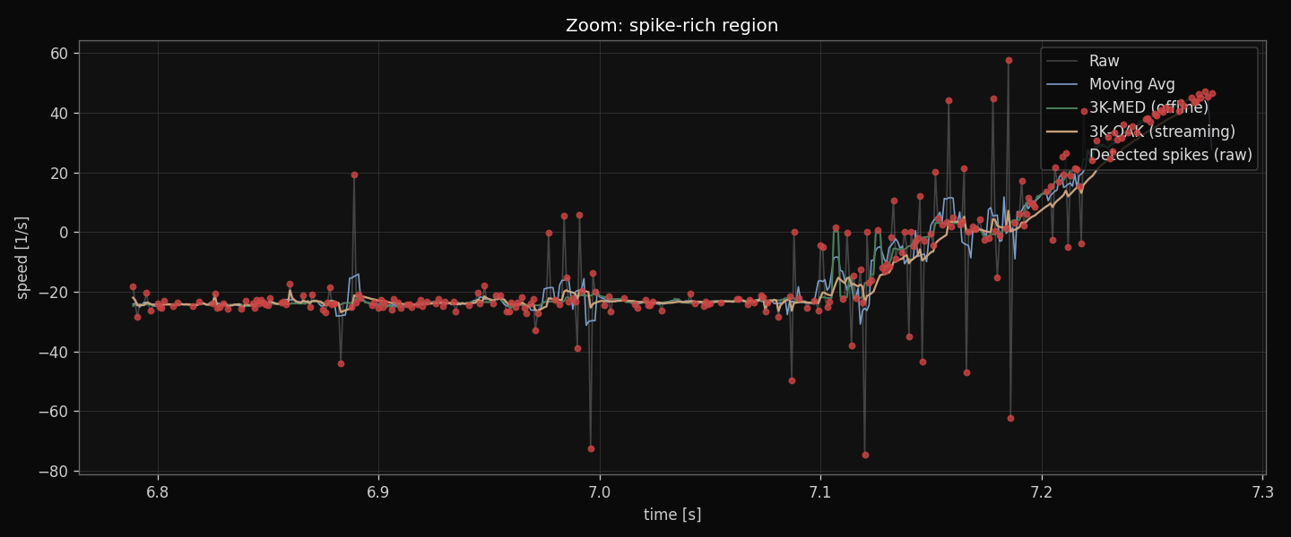
Classical low-pass filters trade noise rejection against lag — the harder you smooth, the further behind reality the controller drifts. Median-based and bilateral filters preserve edges but require a centred window, so they are only usable offline.
The 3K-OAK family addresses both at once: structure-aware streaming filters that detect coherence in the input signal and adapt their smoothing weight per sample. They run inside the control loop on a single sample at a time — no buffer of future values required.
▶ 3K-OAK — Adaptive Structure-Aware Filter
3K-OAK is not pre-tuned to a fixed noise spectrum.
It estimates local signal coherence on the fly and adjusts its smoothing weight per sample — automatically.
11%
RMS reduction vs raw
< 100 B
State per channel
Self-adapting
No per-installation tuning
Streaming, single-sample, no look-ahead — designed for real-time control loops on embedded MCUs. Reference implementation available under NDA for evaluation partners.
Reference Test Case — Industrial Drive Signal
Bidirectional rotational speed signal from an industrial drive controller, 1 kHz logging, ~7 s sequence, ±75 Hz mechanical range. All filters run on the same input, same metric definitions. Tracking error measured against the commanded setpoint.
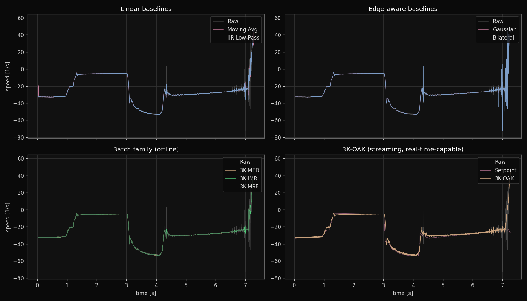
| Filter | RMS tracking error | Spike attenuation | Real-time / streaming? |
|---|---|---|---|
| Raw signal | 7.29 | — | — |
| Moving Average (k=5) | 6.93 | 89.5 % | yes |
| IIR Low-Pass (α=0.3) | 6.87 | 86.1 % | yes |
| Gaussian (σ=2) | 6.94 | 96.2 % | no — needs look-ahead |
| Bilateral | 7.27 | 90.4 % | no — centred window |
| 3K-OAK (streaming) | 6.49 | 47.4 % | yes |
Among real-time-capable streaming filters, 3K-OAK achieves the lowest tracking error (~6 % below the next-best streaming method, ~11 % below raw). Spike-attenuation appears lower because 3K-OAK deliberately stays close to the raw signal to minimize lag and waveform distortion — over-smoothing trades against tracking error. Where look-ahead is allowed and offline post-processing is acceptable, classical batch filters can push spike-attenuation past 95 % at the cost of latency.
Method & Integration
- · Single-sample step function — drops into existing control loops
- · Coherence-aware adaptation — smooths flat regions, preserves edges
- · Bounded by construction — no tuning trap, no instability mode
- · No FFT, no training data, no per-installation tuning
- · Float32, deterministic, ANSI-C-compatible
Reference benchmark run at 1 kHz on industrial drive data. Sample-rate independent up to controller bandwidth. State footprint < 100 bytes per channel. Reference Python implementation for benchmarking; C port on request under NDA.
Solver Technology
Engineering simulations fail silently. Runs can spend hours producing wrong answers before anyone notices.
We build tools that catch this early and rescue simulations that would otherwise fail completely.
Read more...
We build tools that catch this early and rescue simulations that would otherwise fail completely.
Modern engineering relies on simulation: crash tests, fluid flow, heat transfer, electromagnetic fields, structural analysis. Every simulation is an iterative numerical process that either converges to a correct answer, stalls silently at a wrong answer, or fails to finish at all.
Two silent failure modes cost significant engineering time: simulations that report convergence but actually stalled, and matrix problems that fail outright.
Our tools address both. Convergio detects which convergence state a simulation is actually in. CAP solves matrix problems that standard preconditioners cannot.
▶ Convergio — Open Source
Your solver finished 3000 iterations ago. Convergio tells you when to stop — and when something is wrong.
PyPI
Live Package
6
States
MIT
License
result = detect(residual_history, residual_target=1e-8)
# returns: "converged" · "stalling" · "oscillating" · "diverging"
▶ Convergio Enterprise
- · Single header: convergio.hpp
- · Zero dependencies, zero config
- · Real-time: watch() inside your solver loop
- · Post-hoc: detect() on completed runs
- · Adaptive regime detection
▶ CAP — Canonical Attractor Preconditioner
CAP does not optimize the solver iteration.
It restructures the problem so iteration converges by construction.
7
Saddle-point systems ILU(0) cannot factor — CAP converges
5
Ill-conditioned SPD where ILU(0) also fails — CAP converges
952k
Largest solved (ldoor; ILU(0): 18 min, no convergence)
1e-8
Convergence tolerance
Reference implementation available under NDA. Commercial evaluation licensing on request.
Read the table against the standard baseline: ILU(0)-preconditioned CG/GMRES — the standard drop-in preconditioner — run under conditions identical to CAP: same right-hand side (b = A·1), x₀ = 0, tol = 1e-8, iteration budget min(8000, 2·N), same machine, GMRES restart 50.
"Cannot factor" = classic ILU(0) breaks down on the zero pivots of indefinite / saddle-point systems — this is structural, not a tuning artefact. Iterations and walltime are reported separately; CAP is single-threaded.
| Matrix | Standard preconditioner: ILU(0) | CAP (v0.8.3) | Verdict |
|---|---|---|---|
| Tier 1 — standard drop-in ILU(0) breaks down or fails in budget · CAP converges | |||
| d_pretok · 183k · saddle (29% Lagrange) | cannot factor (zero pivot) | 5,380 it | ILU(0) ✗ · CAP ✓ |
| aug3dcqp · 36k · saddle (22% Lagrange) | cannot factor (zero pivot) | 1,000 it | ILU(0) ✗ · CAP ✓ |
| cavity10 · CFD saddle | cannot factor (zero pivot) | 84 it | ILU(0) ✗ · CAP ✓ |
| cavity16 · CFD saddle | cannot factor (zero pivot) | 173 it | ILU(0) ✗ · CAP ✓ |
| cavity05 / 17 / 20 · CFD saddle | cannot factor (zero pivot) | 35 / 109 / 392 it | ILU(0) ✗ · CAP ✓ |
| ldoor · 952k · automotive SPD | FAIL — 8,000 it / ~18 min | 1,455 it / 250 s | ILU(0) ✗ · CAP ✓ |
| bcsstk36 | FAIL — 8,000 it | 3,188 it | ILU(0) ✗ · CAP ✓ |
| bcsstk25 | FAIL — 8,000 it | 203 it | ILU(0) ✗ · CAP ✓ |
| bcsstk13 | FAIL — 4,006 it | 408 it | ILU(0) ✗ · CAP ✓ |
| bcsstk09 | FAIL — 2,166 it | 43 it | ILU(0) ✗ · CAP ✓ |
| Tier 2 — both converge · CAP needs fewer iterations | |||
| bcsstk17 | 7,078 it | 389 it | ~18× fewer |
| ct20stif | 7,104 it / 52 s | 434 it | ~16× fewer |
| bcsstk15 | 504 it | 75 it | ~7× fewer |
| bcsstk14 | 251 it | 54 it | ~5× fewer |
| bcsstk38 | 899 it | 202 it | ~4× fewer |
| thermal1 · 83k | 504 it | 120 it | ~4× fewer |
| thermal2 · 1.2M | 1,838 it / 80 s | 429 it | ~4× fewer it |
| apache2 · 715k | 786 it / 15 s | 399 it | ~2× fewer it |
| bcsstk18 | 368 it | 184 it | ~2× fewer |
| nos4 / nos6 / bcsstk34 / ex5 | 23 / 25 / 47 / 17 it | 1 / 12 / 29 / 2 it | CAP fewer |
| offshore · 260k | 59 it / 0.9 s | 40 it | comparable |
| bcsstk08 / 10 / 11 / 16 / 28 | 25 / 165 / 467 / 40 / 736 it | 14 / 167 / 382 / 35 / 582 it | comparable |
| msc10848 · thermomech_TC | 1,900 it · 8 it | 1,845 it · 7 it | tie |
| Tier 3 — honest limits · standard ILU(0) wins or solves what CAP does not | |||
| nlpkkt80 · 1.06M · KKT | SOLVED — 3,950 it (res 9.9e-9) | res 1.7e-7 — not solved | ILU(0) wins |
| c-68 … c-72 · penalty-KKT | SOLVED — 139–810 it | diverges (auto-flagged) | ILU(0) wins |
| FEM_3D_thermal1 · 18k | 9 it | 735 it | ILU(0) wins |
| bcsstk26 | 210 it | 1,728 it | ILU(0) ~8× fewer |
| bcsstk24 / s3rmt3m3 / bcsstk27 | 177 / 398 / 21 it | 488 / 1,313 / 64 it | ILU(0) ~3× fewer |
| mario002 · 390k · mixed-FE | cannot factor (zero pivot) | worse than baseline | neither — known limit |
| Neither preconditioner converges | |||
| ex11 | FAIL (no-precond CG: 7,325 it) | FAIL | bare Krylov wins |
| bcsstk35 / thermomech_TK / qa8fk | FAIL | FAIL | both fail |
| cavity26 · CFD saddle | cannot factor (zero pivot) | FAIL | both fail |
Reproducibility
The ILU(0) baseline is independently reproducible — the exact harness and recipe for the public SuiteSparse matrices are available on request, so the baseline numbers can be verified without trusting us. CAP itself (v0.8.3) is verified directly on your matrices under NDA. No third-party-validated runs yet.
The Core Value Proposition
CAP is not a universal speed-up: on well-behaved SPD where ILU(0) already works it is sometimes comparable or slower (Tier 3 shows where ILU(0) wins outright, including penalty-KKT and nlpkkt80, which standard ILU(0) solves and CAP does not). These systems are not unsolvable in general — sparse direct solvers with pivoting (MUMPS, PARDISO, UMFPACK) and hand-built block-Schur / augmented-Lagrangian preconditioners handle them in production FEM/CFD stacks. CAP's claim is narrower: a header-only, dependency-free drop-in that converges on these cases without a direct factorization (memory) or a hand-built block preconditioner — where the standard drop-in (ILU(0)) cannot.
Radar Signal Processing
Automotive radar sees things that aren't there. These "ghost targets" cause false braking and dangerous driving decisions.
We filter them out — in software, on the existing hardware, in real time.
Read more...
We filter them out — in software, on the existing hardware, in real time.
Modern cars rely on radar for autonomous driving. Radar sensors measure reflections — but in real traffic, signals bounce off multiple surfaces before returning. These multipath reflections create "ghost targets" that appear real but correspond to no actual object.
Our filter — 3K-PINE — is deterministic: no training data required, no retraining when sensor or scene changes.
▶ 3K-PINE — Multi-Scale Persistence Pre-Filter
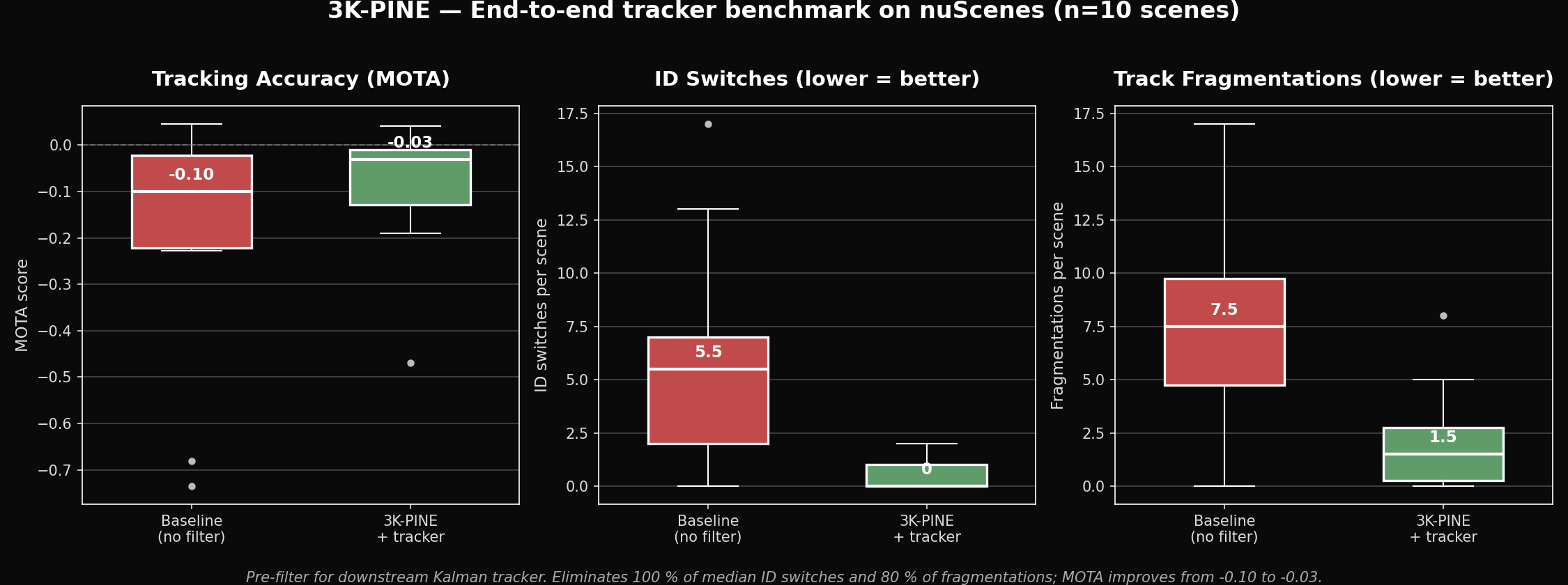
0
Median ID switches
−80%
Track Fragmentations
+0.07
MOTA improvement
End-to-end tracker benchmark on nuScenes v1.0-mini (n = 10 scenes, RADAR_FRONT). Reproducible pipeline; reference library available under NDA for evaluation partners.
Comparative Benchmark
End-to-end tracker pipeline on nuScenes v1.0-mini (n = 10 scenes). Each scene runs both pipelines side-by-side: raw radar → DBSCAN → Kalman tracker versus raw radar → 3K-PINE → DBSCAN → Kalman tracker, evaluated against ground-truth trajectories with CLEAR-MOT metrics.
Technical Approach
Method. Multi-scale temporal persistence combined with signal-coherence analysis. Detections without consistent multi-scale support are rejected as ghost artifacts. The filter is deterministic — no training data required, no retraining when sensor or scene changes.
Position in the stack. 3K-PINE is a pre-filter for the customer's existing tracker. It cleans the detection stream so that the downstream Kalman / JPDA stage spawns fewer false tracks, suffers fewer ID switches, and produces more stable trajectories. Adaptive threshold profiles per operating regime.
All filter parameters are tunable per sensor model and operating regime. Configuration profiles provided for evaluation partners.
- Input. Standard automotive radar detection stream (position + velocity + intensity).
- Output. Filtered detections with persistence metadata for downstream tracker integration.